Supply, demand and willingness-to-pay
Negative oil prices
and other economic stories
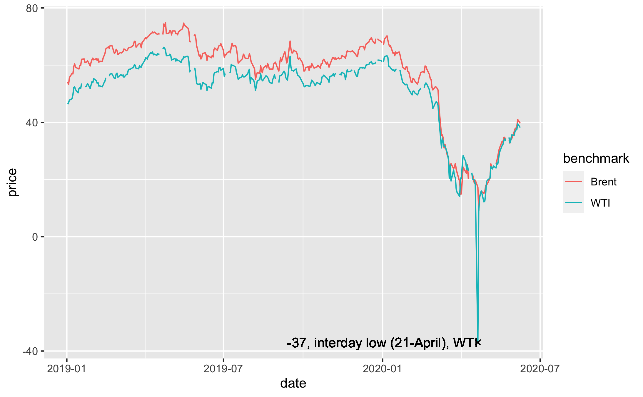
On April 20th 2020 the price of crude oil in the US dropped to -37 dollars a barrell. Actually, we need to be more specific. The futures contract for may delivery of West Texas Intermediate grade crude oil at Cushing, Oklahoma dropped to -37 dollars a barrell. This means that holders of crude oil needed to pay someone 37 dollars per barrell to take it off their hands. This sounds incredible.
The oil price drops to -37 dollars
What happened? You may recall that in first months of 2020, the world started hearing about a a new Corona virus. Health systems from China to Italy to New York City started buckling under the pressure. And governments around the world started advising, and then ordering their citizens to stay at home.
Consequently the demand for crude oil, which powers much of the world's cars and airplanes, dropped. Supply and demand for crude oil usually varies. Consumption can pick up during some times of the year, like during the summer driving season in the US. Production may drop off in periods with stormy weather in the Gulf of Mexico. To smooth out these variations, the industry uses storage.
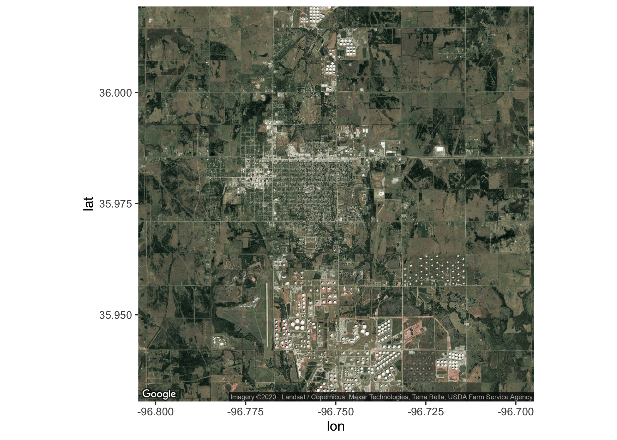
Below is a picture of Cushing, Oklahoma from Google Maps. This is one of the world's largest crude oil hubs. Here, many of the US's largest oil pipelines cross. Producers of crude oil will generally deliver their oil here when they have agreed upon a price in the futures market. All of the white dots you see around are large storage tanks. Just in this one town, there are millions of liters of storage space.
Cushing, Oklahoma in the US.
But when lockdown orders and travel restrictions began to take hold, the demand for fuel fell so fast that the market and available storage was not able to adjust. Producers of oil had sold contracts for delivery months in advance, so they continued to produce. Refiners who buy the crude oil in order to turn it into petrol, diesel and other finished products were not buying however. Storage tanks were quickly filling, and there were stories of using everything from filling up tanker ships to above-ground swimming pools.
But after all the alternatives were exhausted, you still had some traders who held legally binding futures contracts to buy crude oil in may, but who had no one to buy it and no place to store it. At the most desperate point, on April 22nd, some of these traders were willing to pay 37 dollars per barrell for someone to take the crude oil off their hands.
Eventually, the market came back into a sort of equilibrium at a low, but positive price. Production from oil wells was reduced and refineries were able to slowly start using up their inventories of stored crude oil. Markets are often messy and complicated, like the market for crude oil. Yet, the stylized models of supply and demand that we develop in these lectures can go a long way in helping understand why markets behave the way they do.
This introductory lesson gives an overview of supply and demand concepts that you have hopefully seen before. In the following lessons, we dig deeper into the theory and show how we can interpret supply and demand curves at both the individual level and market level.
The demand curve
We can write a general formula for a linear demand curve as:
$$P=c-dX^D$$
The demand curve shown in the figure above can be written. (When we write the equation with price on the left-side, we often refer to it as the inverse demand function.)
$$P=300-0,5*X^D$$
The slope of the curve is \(d=0,5\)
This says that if the price goes up by 10, then quantity demanded would go down by 20 (\(\frac{10}{20}=0,5\)).
We can interpret 300 as the price required to get to exactly 0 in demand. If we have a price that is 300 or higher, then no one wants our product.
You can try putting in your own values of c and -d:
The supply curve
We can write a general formula for the supply curve as:
$$P=a+bX^S$$
The supply curve we have shown in the figure can be written:
$$P=40+0,5*X^S$$
The slope of the figure is b (\(b=0,5\))
This says that if the price goes up by 10, then the quantity supplied increases by 20 (10/20=0,5)
We can interpret 40 as the price when the amount supplied is exactly 0. Any price that is 40 or lower will lead to no producer willing to supply a given product.
You can put in your own values for a and b:
Market equilibrium
Mathematically, we can find our market equilibrium by taking our equations for demand and supply and setting them to be equal to each other.
$$P^D=c-dX^D$$ $$P^S=a+bX^S$$
The equilibrium condition is that the prices (\(P^D, P^S\)) and quantities (\(X^D, X^S\)) are the same. We will now leave out "D" and "S" superscripts since in equilibrium the price (and quantity) of supply and demand will be equal.
$$c-dX = a+bX$$ $$X^{*} =\frac{c-a}{b+d}$$
We use "*" to signify that this is the equilibrium value.
To find the equilibrium price, \(P^{*}\), we have to plug in \(X^{*}\) in either the supply or demand curve.
Here we will do it with the demand curve:
$$P^* = c-dX^{*}$$ $$P^* = c-d\frac{c-a}{b+d}$$ $$P^* = \frac{cb+da}{b+d}$$
Try it:
Find the equilibrium values for the following supply and demand curves:
$$P^S=40+0,5*X^S$$ $$P^D=300-0,5*X^D$$
Shifts in supply and demand
Shift in demand
Shift in supply
Quiz
Answer True or False about the following statements:
Individual supply curves
Marginal willingness-to-pay
When we look at the individuals demand curve, we can interpret the curve as marginal willingness-to-pay.
Marginal willingness-to-pay means how much (in theory) you are willing to pay to get one more of a certain good (let's say apples).
Our demand curve still has a negative slope. This comes from the assumption that you value the first apple you buy highly. But after having eaten one apple, you value the next apple somewhat less. After you have eaten 100 apples in a week, perhaps the marginal value you place on one more apple is very low.
When we are looking at individuals, we often model the supply curve as a horizontal line. Meaning, you can go to the store and buy as many apples as you want for exactly the same price.
Press Increase quantity. We see the situation where when we only buy a few apples, each one of those apples is valued quite highly (our willingness-to-pay is the vertical distance.) Luckily, the price at the store (the horizontal supply curve) is lower than your willingness-to-pay. We can consider the difference between how much we are willing to pay and how much we actually pay as a form of surplus - we call it consumer surplus.
Nå har vi kjøpt and spist noen bananas, ønsker vi å kjøpe flere? Vi ser på vår etterspørselskurv (marginalbetalingsvilje), and ser at den ligger fortsatt høyere en prisen på butikken. Vi får fortsatt mer glede av å kjøpe and spise eplene enn det de koster. Vi fortsetter å trykker på Øk mengden.
When do we stop buying apples?
When our enjoyment of an extra apple (our marginal willingness-to-pay/demand curve) is no longer more than the price at the store (the horizontal supply curve), then we stop.
The blue triangle that is formed at this equilibrium is the total consumer surplus.
If we press Increase price or Reduce price we see how both the equilibrium quantity and total consumer surplus changes with a changed price.
Income, normal and inferior goods
Price is obviously not the only variable that decides our demand. Our income is also important. But our demand for different goods are affected in different ways by a change in income.
When we are done being a student and start working and making a full-time income, we may stop buying as much frozen pizza and spend more money at restaurants. So increased income can mean either more or less consumption of a given good, depending on our preferences.
We define a normal good as a good you buy more of when your income increases. A inferior good is a good you buy less of when your income increases.
Below, answer whether the following goods are most likely normal or inferior. Of course, whether a good is normal or inferior depends on every persons individual preferences. Some people love frozen pizza and will buy more when their income increases. But think in terms of averages over a population. You can also think in terms of quality, rather than just quantity. When your income increases, you may buy a nicer apartment rather than more apartments.
Cross-price effects
Sometimes our demand for a certain good is influenced by the price of one or more other goods.
If the price of hotdogs increases, then we will likely also eat less ketchup. Hotdocs and ketchup are Complimentary goods.
If the price of a buss ticket increases, you may decide to purchase an electric bike. Taking the bus and an electric bike are alternative goods.
In the following answer if the goods are most likely complimentary or alternative goods. Again, think on average over most people as individual preferences can always diverge.