Fixed and variable costs
Fixed costs and the world's most important car factory.
As we've already talked about, an important factor that differentiates different assumptions about a production function is the time perspective. The difference between a short-run model and a long-run model is whether there is enough time to build out a new factory, or install new machinery.
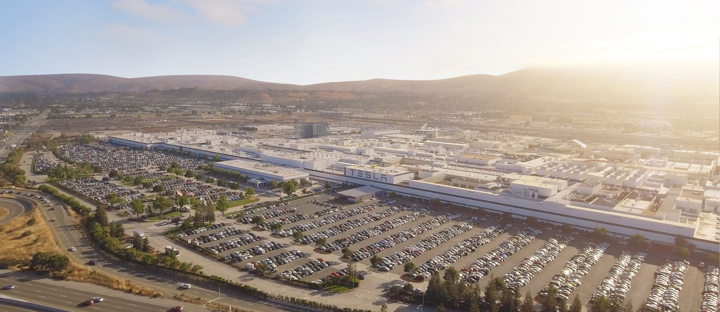
Tesla's first full-scale factory is an interesting case study. Tesla bought the factory immediately after the financial crisis of 2008-2009. They bought the factory from GM and Toyota, who had worked together on building the factory and producing cars there in the 1980's. The factory was initially called NUMMI - New United Motor Manufacturing Inc.
Toyota was motivated to invest in the project in order to gain better access to the US market, and to avoid growing worries about protectionism. But it was perhaps GM that would get the most out of the cooperation. During the 1980's, Toyota and other Japanese auotmakers looked like they were well on their way to outcompeting their US competitors. They produced inexpensive, petrol-sipping and highly reliable cars at a time where US producers were producing gas-guzzling monsters with a tendency to break down. GM especially interested in learning about Toyota's revelotionary production technique that has become known as learn manufacturing.
One aspect of this new manufacturing process is what the Japanese called "Jidoka." This is an idea about how to introduce automation in factories in a way that is driven by human production. A production line is first primarily composed of workers who try to experiment and optimise a process. Only then are manufacturing robots and machinery introduced in order to automate and improve the efficiency.
Another concept was the "Just-in-Time" process for minimising the amount of inventory on hand. This included both inventory of parts and raw materials as well as the production cars. The ideas was to adjust production to the number of current orders one had at any given time, so that you didn't end up producing many cars that you weren't able to sell. A factory would then also adjust it's levels inventory for parts and raw materials to match the production levels. Toyota had discovered a manufacturing technique that allowed for flexible, low cost manufacturing that also led to high-quality products.
Putting on our microeconomic hats, we could say that even if Toyota and GM had the same amounts and quality of labor and capital, Toyota had higher total factory productivity. They were able to combine capital and labor in order to create cars in a more efficient and profitable way. GM was very interested in learning these techniques, as were all the other major car companies. Lean manufacuting spread, and is now standard not just in automobile manufacturing, but in almost all production firms.
It seems appropriate then that the next big revolution in the car industry would also start in the old NUMMI-factory. In this factory Tesla would produce the world's first truly mass-produced electric car: The Model S, and eventually the Model 3.
Tesla was able to get production up and running at their factory, though not without problems.
The interactions between fixed costs and production are important for understanding modern manufacturing, and it is something we will look at in this lesson.
Fixed costs
Fixed costs and production in the short-run.
From the perspective of a firm, what often differentiates the short-run from the long-run is the the possibility of building out more capital.
If a firm suddenly gets a big increase in demand, then it is usually impossible to just build a new factory. It takes time to arrange financing, find a location, planning and construction.
This is why we often think of capital investments as fixed in the short run.
When we consider production and costs in the short-run, there are often some costs that we account for differently and affect our decisions differently because we incurr those costs no matter how much production we plan on having: What we called fixed costs. Considering a car company, we should of course consider the cost of a factory when calculating the total cost of a car. But whether that factory produces 1000 or 1010 cars in a given day probably doesn't change the cost of that factory.
Consider the figure above on top: We see that the figure doesn't start at 0 on the vertical axis, but rather a bit higher - these are the fixed costs, the costs we have to pay even if we set production to 0 in a certain day.
In the lower figure we show several metrics for costs per unit.
The simplist metric is average costs. Here we just divide total costs with the number of cars produced. We see that this measure starts very high, since we are dividing all of the fixed costs by just a few units of production - let's call them cars to be concrete.
Another line is the marginal cost: the cost of making one extra car. This increases linearly. As we've seen earlier, this comes from an assumption that our production function has diminishing returns to scale.
For our average cost curve, we see that the curve initially slopes downward, reaching a bottom and then begins to increase. You can think of the average cost curve as a trade-off between the effects of spreading the fixed costs over more production, which brings down average production costs, and increasing marginal costs.
Where exactly the minimum value of average costs? We notice that it is where the marginal cost curve crosses the average cost curve. We can interpret this as saying that as long as the costs of producing one more (marginal costs) is lower than the average costs, then the average costs are brought down by producing one more.
We can also show the average costs where we have taken out the fixed costs. These are the average of the costs that vary with production, we call this variable average costs
Why does this lie under the marginal cost curve?
Because marginal costs are always increasing, so producing one more car will always be more expensive than the average variable costs of producing all the previous cars.
Fixed costs and production in the short run: Mathematically.
We can write total costs as:
$$C(y) = C_v(y) + F$$Where \(C_v(y)\) is the variable costs and F represents the fixed costs. Notice that F is not a function of production, \(y\), this is the definition of fixed costs.
We can find the marginal costs by taking the derivative:
$$C'(y) = C_v'(y)$$Variable average costs can be written as:
$$\frac{C_V(y)}{y}$$Fixed average costs can be written as:
$$\frac{F}{y}$$And total average costs is:
$$\frac{C(y)}{y} = \frac{C_V(y)}{y} + \frac{F}{y}$$Contribution margin
Profit maximization and contribution margin
In the figure we now show only marginal cost and the market price, p.
We recall from lesson 11 that a firm that wishes to maximize profits will produce until marginal costs are like price. We decide to produce one more car as long as the cost of that extra car does not exceed the price that car will get on the market.
We can also explain this with a concept from management accounting: Contribution margin. This is the difference between the marginal cost of producing a unit and the market price. We can think of this as the part of the sales price that goes towards paying down fixed costs and/or adding to profits. When a firm manager is trying to decide on whether to make an investment, they often need to consider whether the contribution margin will be large enough to merit the extra fixed costs.
Press the Increase production button. We see that the Contribution margin per car becomes smaller and smaller because the marginal cost increases. But we continue to produce until we have 0 in contribution margin.
We can define contribution margin mathematically.
We start by defining profit as the difference between total revenues and total costs:
$$\pi(y) = py - C_v(y) - F$$We take the derivative in order to find the level of production that maximizes profit.
$$\pi'(y) = p - C'_V(y) => p=C'_V(y)$$So now we are back to our old condition for optimality: Price = Marginal cost. Fixed costs drop out - they are not important in deciding the level of production.
When should you quit? The supply curve and sunk costs
Until now we have talked about fixed costs like a car factory. But we can think about different types of fixed costs and how those different types of fixed costs affect how we make decisions in our firm.
A car factory is to a high degree irreversible. That means that when we have built that factory, it is in large part only useful for the car company that built the factory. It would be hard to go and sell it to another company. Another company--even another car company-- would need to rebuild large parts of the factory in order to be able to produce their product.
A factory is also characterized by the fact that it is independent of production. When we have built a factory, then we have to pay for that factory even if our production is zero. The combination of being irreversible and independent of production (including 0 production) makes a factory what an economist calls a sunk cost. After we have decided to build the factory and paid for it, then we can't go back and change that decision, so it becomes irrelevant for any subsequent decisions on how much we should produce or whether we should produce at all.
On the other hand we have production-dependent fixed costs. These are still fixed costs in the sense that they do not change with differing levels of production. But if we stop production completly, then we can also avoid these costs. We can think of a lot of administrative costs as being production-dependent fixed costs. You may need a receptionist at the front desk of a factory, and that cost doesn't change whether you are producing 10 or 1000 units at that factory. But if you decide to shut-down the production, you can also fire the receptionist.
The difference between sunk costs and production-dependent fixed costs will affect how we model our supply curve, which we demonstrate below.
The supply curve and production-dependent fixed costs
In the top figure above we show two cost functions. In the lower curve we only include fixed costs that are irreversible and independent of production -- what we call sunk costs.
The top cost curve also includes production-dependent fixed cost (like the receptionist at the factory).
In the bottom figure, we have divided both cost curves by production (y) to give a measure of average costs with production-dependent fixed costs (yellow) and average costs that includes both sunk costs and production-dependent average costs (orange).
Now we will ask a question again: How much with the firm produce and sell for each price? In other words, what is the supply curve for the firm?
Press the Increase price button: The dashed line represents the market price.
Without fixed costs we could just follow the marginal cost curve and used that to decide how many units (cars?) we produce.
But looking at the average cost curve that includes production-dependent fixed costs, we see that at a low market price, we will lose money on each car we produce, even if the price is above the marginal cost of production.
In other words, when we take into account the production-dependent fixed costs (like the receptionist at the factory), then we would be better off to stop production. (But notice that the sunk costs play no role in our decision.)
Therefor the first part of our supply curve is drawn as a vertical line at 0 (thick blue line).
Continue to press the the Increase price button: When the price comes over the yellow curve, then we can produce enough cars at high enough prices such that we can cover the production-dependent fixed costs. Therefor, we are willing to start production and now our supply curve follows our marginal cost curve.
Still, if the price is between the yellow and orange average cost curve, we will in total lose money. So why are we still willing to produce cars? Because the factory costs are sunk. We can't get that money back even if we stop production, so it becomes irrelevant in the decision on whether to produce or not.
Quiz
Answer True or False about the following statements
Problems
-
Let us say we have a total cost function:
$$C(y) = 0,5*y^2 + 50$$a.) What are the firms fixed costs?
b.) Write an equation for the firms marginal costs.
c.) How much production does the firm need in order to reach mimimum average costs?
a.) The companies fixed costs are 50.
b.) Marginal costs can be written as the derivate of the total cost function, (C(y)):
$$C'(y) = y$$c.) Average costs are lowest where the average cost curve meets the marginal cost curve:
$$\frac{0,5y^2+50}{y} = y$$ $$0,5y^2 + 50 = y^2$$ $$50 = 0,5y^2$$ $$y^2=100$$ $$y= \sqrt{100} =10$$ -
a.) The contribution margin is the difference between the price and marginal cost:
$$p-C'(y) = p-y = 12-10=2$$b.) We can write our profit function as:
$$\pi(y) = p*y - C(y) = 12y - (0,5y^2+50)$$We take the derivative and set to zero in order to find the maximum:
$$\pi'(y) = p - y = 0$$ $$y=p=> y=12$$We can then calculate the contribution margin of each unit we well:
The first unit had a marginal cost of 1 and with a market price of 12 we get a contribution margin of 11.
The second unit had a marginal cost of 2 and thus we get a contribution margin of 10, and so on.
Adding up, we get
$$11+10+9+8+...+0 = 66$$Subtracting our fixed costs:
$$66-50=16$$We find we get a total profit of 16.
Alternatively, we could have just plugged in our optimal production back into our profit function:
$$\pi = 12*12 - (0,5*12^2 +50) = 22$$But here our answer is a bit different, why? Because this gives an answer where we assume we can split up our production into fractions.
-
Now we change our total cost function to:
$$C(y) = 0,5*y^2 + SC + PDC$$Where SC stands for Sunk Costs and PDC stands for production dependent costs:
$$SC=25$$ $$PDC =25$$a.) How much does the market price need to be before we start production?
b.) How much does the market price need to be for us to have a positive total profit?
To start production, the price must be high enough that we cover our variable costs as well as our production dependent costs
We can write our condition as:
$$p*y = 0,5y^2 +25$$Our condition for setting the level of production is to set price equal to margina cost:
$$p=C'(y) => p=y$$Combining the equations above:
$$p^2 = 0,5p^2 + 25$$ $$0,5p^2 = 25$$ $$p^2 = 50 =>p=\sqrt{50} \approx 7.07$$The price must be at least 7.07 to start production
b.) We will first get a profit when total revenues are above total costs:
$$p*y = 0,5y^2 + 50$$Inserting into our condition for maximum profits:
$$0,5p^2 = 50$$ $$p^2 = 100 => p=10$$The price must be at least 10 in order to get non-zero profits.
(notice that this is also where we have the minimum of average costs)
Using the same cost curve as above:
$$C(y) = 0,5*y^2 + 50$$And now we also know the market price, p=12.
a.) What is the contribution margin on the 10th unit we produce and sell?
b.) If we wish to maximize our profit, how much should we produce? Will our total profits be positive?