Economies of scale

From growing pains to mass production

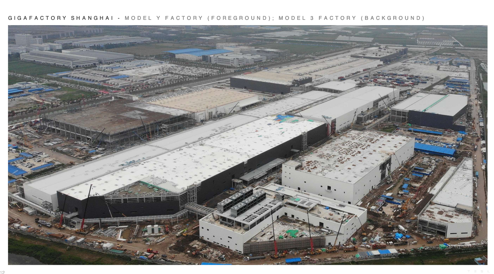
In the last lesson we discussed how Tesla experienced problems when they wanted to ramp up production of their Model 3 sedan. They ended up with high marginal costs for the first cars that were produced.

At the same time we know that scaling up their production was seen as necessary for Tesla to survive in the long run. How can we reconcile these two seemingly contradictory thoughts? On the one hand, higher production leads to higher marginal costs, but we need higher production to bring down average costs.

The solution is to consider different time scales. In the short-run, where we consider much of our capital (factories, production machines, etc) fixed, increasing production can lead to higher marginal costs. But at a longer timeframe, we can build new factories, optimize our processies and learn from our experiences, all which let us expand production while bringing down the average costs of our product. With more production, we can divide some fixed costs over more cars: This includes such immaterial costs like design, marketing and administration.

Tesla has always been aware of these *economies of scale*. In 2016 they built what they called a gigafactory for battery production near Reno Nevada. Such large scale battery factories have now become the norm for the quickly expanding electric car industry.

Despite increasing competition, Tesla is still a leader in battery and electric motor technology. The large scale of their operations and efficient and vertically integrated operations is seen as a way of keeping their costs lower than their competitors.

In this lesson we take a theoretical look at production in the medium and long term. We assume that a company is able to increase production without marginal costs increasing. We will also make explicit the connections between a companies profit function and a companies supply curve.

Constant economies of scale

Increase input avg. prod Increase productivity

Constant returns to scale

We recall from lesson 9 that with our Cobb-Douglas production function, when we increased both capital (K) and labor (L) proportionally, then we got constant returns to scale: If we doubled both capital and labor, then we doubled our production.

In the figure above, we can see a simple model of constant returns to scale. The model can be written simply as \(y=A*v\), where A represents productivity. Previously we called this total factor productivity, but in this model there is only one input factor, so there is no difference between productivity from more capital and total factor productivity.

We start with setting A=1. That means that if we add 100 of our resource input v then we get 100 in production. Press the Increase input button. We see that when we increase our resource input, $v$, then our production increases proportionally.

What is our marginal productivity in this calse?

It is A! If we increase our input with 1, then we get A=1 in extra (marginal) production

What about average production?

Press the avg. production button.

We can see that when we have constant returns to scale, then there is no difference between average productivity and marginal productivitiy - both are A.

The cost function

The cost function with constant returns to scale is also simple.

We recall that the cost function is just the transformation of our production function: We invert the production function and then multiply by the price for our resource input.

First we invert our production function:

$$y=Av =>v=\frac{y}{A}$$

Then multiply by our input price, q

$$C = q*\frac{y}{A}$$

The cost function has a simple interpretation: The higher our productivity, A, the lower the costs.

The marginal and average costs are also simple to compute.

To produce an extra unit of production, we need \(\frac{1}{A}\) units of our resource input. Multiplying by the price, $q$, of our resource input, we get: \(\frac{q}{A}\)

Again, when we have constant returns to scale, there is no difference between average and marginal productivity.

The profit function

We can take a final step by taking our production and cost functions and creating a profit function. All we need is a constant price of our production: p

$$\pi = p*y - C $$ $$\pi = p*y - \frac{q*y}{A}$$ $$\pi = (p-\frac{q}{A})*y$$

Here we have a simple interpretation: For each unit produced, our profit increases by the difference between the price and cost of production.

The supply curve

Now that we have spent some time considering how to model production and costs from the perspective of a firm, we can start to think a bit deeper about what a supply curve represents.

The supply curve represents how much of a product a firm is willing to supply on the market for a given price.

Intuitively, the supply curve should then be closely related to the cost curve.

We start by considering the simple cost curve we discussed above that comes from a production function with constant returns to scale.

Supply curve with constant returns to scale

A production function with constant returns to scale means that the cost of producing an extra unit is the same no matter the total production level.

The supply curve for a company with constant returns to scale is represented by a horizontal line that lies at the marginal cost \(\frac{q}{A}$\)

We can then ask, how much a firm with a given production function with constant returns to scale is willing to produce and sell for various prices.

A reasonable principle might be that we do not want to produce and sell a unit if it costs more to produce it than we get in extra revenue (the price) from selling it.

What if the market price is above the marginal cost of production?

In that case the firm would be willing to produce as many as the market demanded.

That's why the supply curve of a firm with constant returns to scale and constant marginal costs is a horizontal line.

The supply curve with diminishing returns to scale

Increase price

We recall from lesson 10 that with diminishing returns to scale we got marginal costs that increased with production: The more we produced, the more it cost to make one more unit.

We can think about this as a short-term model: Given the capital (factories, machines) that we have, then increasing production will cost more per unit we increase: We have to pay overtime, machines get worn out quicker, etc.

So how much should we produce and sell?

In lesson 10, we established that we should produce up to the point where marginal cost was equal to marginal revenue..

In the figure above this is represented by where the market price (marginal revenue) is equal to the marginal cost curve.

Now press the Increase price button. When the market price has increased, then we are willing to produce more.

In the figure under we draw a function that represents this relationship. If we continue to press the Increase price button, we will draw a curve that represents what we are willing to produce at various prices. This is the definition of a supply curve!

In this case, the supply curve is exactly equal to our marginal cost curve. But this will not always be the case. Here it is true because we have a constant market price. Later we will see situations where that is not the case.

Quiz

Answer True or False about the following statements.

Problems

1. We have the following production function with constant returns to scale:

   $$y=2v$$

   a.) If the price of the input is q=4, how do you write the cost function?

   b.) What is the marginal cost when y=10, 20 and 30. What is the average cost when y=10, 20, 30?

   c.) If the market price is p=3, should the firm increase production?

   Show answer

   a.)

   Starting with our production function, \(y=2v\) and write it so that v is on the left-hand side:

   $$v=\frac{y}{2}$$

   We get total cost by multiplying by the price of the input, \(c\):

   $$C = q*v= \frac{qy}{2}$$ $$C = \frac{4y}{2} = 2y$$

   b.)

   We have a constant marginal cost: mc=2 no matter production level. Average cost is the same as marginal cost.

   c.) If the price is 3 and the marginal cost is 2, the company will always be able to increase their total profit by increasing production. The company wants to produce as many as they can!

2. Can you write a formula for the supply curve for the firm in problem 1?

   Show answer

   The supply curve is a horizontal line at the level of the marginal cost: mc=2

   We can interpret this supply curve to mean that as long as the market price is 2 or more, the firm will produce as many as it can.

3. Now let's say that a firm's production function can be represented by a Cobb-Douglas function with diminishing returns to scale:

   $$y=2v^{0,5}$$

   a.)If the price of the input is q=4 what is a formula for the cost function?

   b.)Can you write a formula for the supply curve of the firm?

   Show answer

   a.)

   We re-write our production function with v on the left-hand side:

   $$v^{0,5} = \frac{y}{2}$$ $$v = (\frac{y}{2})^2$$

   We multiply by the price on our input, q

   $$C(y) = 4*v = 4(\frac{y}{2})^2 = y^2$$

   c.) With a Cobb-Douglas function, the marginal cost function becomes a linear increasing function:

   $$C'(y) = 2y$$

   To find optimal production, we then need to set P=MC:

   $$p=2y$$

   Which also then becomes the formula for the companies supply curve