Production resources and cost minimization
Robots or humans?
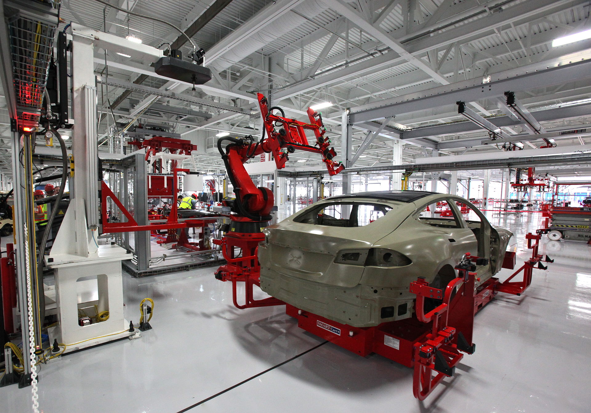
Source: Tesla Annual Report
When Tesla began planning to produce their mass-marked Model 3 sedan, their strategy was to use many production robotos and a high degree og automation in the production process - much more so than the traditional automanufacturers. In this way, the thinking went, they would increase the productivity of the plant and keep costs down.
But the reality of car manufacturing turned out to be more difficult, and Tesla experienced a period of unexpected and expensive production problems.
Tesla eventually realized that they had been to aggressive in their automation strategy. They could get more efficient production and lower costs by having more human labor and fewer robots.
In this lesson, we will model this type of problem: What combination of human labor and capital (machines) gives the most efficient production and lowest costs.
We will see that our microeconomic models often include an assumption that the lowest cost production includes a good mix of labor and capital. But we will also see that when technology improves, we will use capital more intensely.
The Isoquant curve
Up until now we have made an extreme simplification when modelling how a firm decides on their inputs. We have said that a firm simply decides on a certain amount of a "factor input" to produce a certain amount.
Now we are going to add a bit more realism by developing a model where we have two inputs. We want a way to analyse how much we want of each one of these inputs and for that we will make use two new concepts: The isoquant curve and the isocost curve.
The figure above shows an isoquant curve. Perhaps it looks familiar, and that is because mathematically it is identical to the indifference curve we met in earlier lessons.
An indifference curve models a consumers preferences between two goods, showing all the combinations of those two goods that give the consumer the same level of utility.
The isoquant curve represents all the combinations of two inputs that give the same level of production.
If we are thinking about a car factory, the red curve represents a goal for how many cars a firm wishes to produce. To reach that goal, we have to choose different combinations of capital (production robots) and labor (workers).
Press the Increase production button, and notice that the isoquant curve moves out.
Substitution and capital intensity
When we modelled our consumption preferences with an indifference curve, we had an assumption that we usually want a good mix of goods. This assumption was expressed mathematically as having an indifference curve that is concave - that is it bends towards the (0,0) point.
Much the same can be said about the isoquant curve: We can often get more efficient production by having a mix of input factors.
Considering our car factory, In the figure we show two points that show different combinations of robots and workers: We call these points Tesla and Ford. Both lie on the same isoquant curve, which means both companies are producing the same number of cars.
Tesla has more robots-they have chosen a production method that relies more on automation. The economist would say that they have a more capital-intensive production.
For has chosen a combination with more workers, which is less capital intensive but can potentially be more flexible.
We can see here that to a certain extent workers and robots are substitutes. You can replace one for the other in your production process.
The slope of the green line represents the substitution possibilities. That is, how many workers can a robot replace while remaining at the same production level. We call this the Technical Rate of Substitution (TRS).
Press the Increase robots button a few times. We notice that as we increase the number of robots we use in our production, the TRS becomes steeper. We can interpret this to mean that as we try to replace more and more workers, this becomes more and more difficult. There are some tasks that humans are still much better at. This was a bit of the problem that Tesla ran into when it first began mass production of its Model 3 sedan.
Costs and budgets
Just like when we were modelling consumer choice, prices and budgets are essential for the decisions facing firms. We model input prices and budgets facing a firm with a budget curve, though now we will call this a isocost curve.
The line above represents all possible combinations of robots (capital) with a price q and workers who make a wage of w which we use in our production, where we have a total budget of m.
The area in light blue represents all possible combinations of robots and workers that comes under our budget
Press the Increase budget button. We see the isocost curve move outwards. We now are able to buy more of both robots (capital) and workers (labor).
Press the Increase wages button a few times. Here we see that when wages become higher, then we are able to hire fewer workers.
Press the Increase price of robots button a few times. Now we see that we are able to buy in fewer robots.
Cost minimisation
Now we will combine the isocost curve with the isoquant curve to find the point where we produce a given amount at the lowest possible cost.
In the figure we start at a point along the isoquant curve where we have many robots (capital) but very few workers (labor)
Press the Increase workers button: As we have seen before, the substitution possibilities between robots and workers is large. By employeeing just a few extra workers, we can maintain the same level of production but with many fewer expensive robots.
We can continue to press the Increase workers button until the point lies close to the isocost (budget) curve.
Notice the slope of the green line has become less steep. When we hire more employees, we give up fewer robots to keep the same production level.
One of the conditions for cost minimisation is that the slope of our substitution possibilities line (TRS, the green line) is the same as our isocost line (budget line). Why?
Remember that the slope of the isocost curve (budget line) is decided by the relative prices of the two input prices (the price of robots and wages: \(\frac{q}{w}\)
Let us say that is not the case: that the slope of our substitution possibilities line er more than the slope of our isocost curve. Then we know that we could save money by trading our a robot (selling it for q) in order to hire one more worker (which we pay a wage of w), while we maintain the same level of production.
But when our substitution possibilities to exchange workers for robots becomes exactly the same as our relative prices, \(\frac{q}{w}\), then we can no longer reduce our costs by trading robots for workers. This is the definition of our cost minimum.
Now that we have reached our minimum, we see that we can not reach our production goal given our budget for our input factors. Press the Increase budget button until the isoquant curve just barely touches our isocost (budget) line. This is the point with minimum costs but where we still are able to produce our intended amount. There does not exist any other combination of input factors that allows us to produce our goal amount for less.
You can check the answer by pressing the Minimize costs button.
Du kan sjekke svaret ved å trykke på Minimere kostnader
Cost minimization: Mathematically
We can write total production costs as:
$$C(L,K)=wL + qK$$Where L represents labor, K is capital (robots), w is wages (price of workers) and q is the rental price of capital.
If we hold C constant, then we have a formula for our isocost curve.
We can write it as:
$$K=\frac{C}{q} - \frac{w}{q}L$$We can write our production function in general as:
$$y=f(L,K)$$Just like our utility function/indifference from earlier lessons, we can write our production function in various mathematical forms in order to give it wished-for properties. Most commonly, we can write it as a Cobb-Douglas form:
$$y=f(L,K) = AK^aL^b$$Marginal productivity to workers or capital means how much more production we can have if we increase the amount of labor or capital we use by a little bit.
We calculate our marginal productivity by taking the derivative of our production function.
The marginal productivity of labor is then:
$$f_L(L,K) = \frac{\partial f(L,K)}{\partial L}$$If we have a Cobb-Douglas form of our production function, then it becomes:
$$f_L(L,K) = b*AK^a*L^{b-1} = \frac{bAK^a}{L^{1-b}}$$The marginal productivity of capital becomes:
$$f_K(L,K) = \frac{\partial f(L,K)}{\partial K}$$With a Cobb-Douglas this becomes:
$$f_K(L,K) =a*AK^{a-1}L^b = \frac{aAL^b}{K^{1-a}}$$The technical rate of substitution (TRS - the slope of our isoquant curve) can be written:
$$TSB = \frac{f_L}{f_K}$$With a Cobb-Douglas, this becomes:
$$TSB= \frac{f_L}{f_K} = \frac{b*AK^a*L^{b-1}}{a*AK^{a-1}L^b} $$ $$ = \frac{bK^a*K^{1-a}}{aL^b L^{1-b}} = \frac{bK}{aL}$$Cost minimization
To find our cost minimization given a production level, y, we have two conditions:
That the slope of the isocost curve (the input price relationship, w/q) is the same as the isoquant curve (TRS):
$$ \frac{f_L}{f_K} = \frac{w}{q}$$Or with Cobb-Douglas:
$$\frac{bK}{aL} = \frac{w}{q}$$And then we have to check that we are on the isoquant curve:
$$y=f(L,K)$$Or with a Cobb-Douglas:
$$y=AK^aL^b$$
With these two equations/conditions, we have to unknowns \((K, L)\), and we should be able to find a solution.
Quiz
Answer True or False about the following statements
Problems
-
We have a production function for cars that we can write:
$$y=K^{0,5}L^{0,5}$$And we aim to produce 100 cars
Wages are \(w=1\) while renting production robots (capital) costs \(q=1,5\)
a.) What is the TRS?
b.) How many production robots (K) and workers (L) should we use in order to minimize costs?
c.) Workers have managed to negotiate up their wages to \(w=1,5\). How many robots (K) and workers (L) should the firm use now? How much extra will it cost the company? What has happened with the number of workers in the firm?
a.)We define the TRS as:
$$TSB = \frac{f_L}{f_K}$$Where
$$f_L = 0,5K^{0,5}L^{-0,5}$$ $$f_K = 0,5K^{-0,5}L^{0,5}$$ $$TSB = \frac{f_L}{f_K} = \frac{0,5K^{0,5}L^{-0,5}}{0,5K^{-0,5}L^{0,5}}$$ $$= \frac{K^{0,5}K^{0,5}}{L^{0,5}L^{0,5}} = \frac{K^{0,5+0,5}}{L^{0,5 + 0,5}} = \frac{K}{L} $$b.) Our optimal condition is:
$$TSB=\frac{w}{q} => \frac{K}{L} = \frac{1}{1,5}$$ $$K=\frac{2}{3}L$$And we have to make sure we reach our production level:
$$y=K^{0,5}L^{0,5}$$ $$100=(\frac{2}{3}L)^{0,5}L^{0,5}$$ $$100=(\frac{2}{3})^{0,5}L^{0,5}L^{0,5}$$ $$100=(\frac{2}{3})^{0,5}L^{0,5+0,5} =(\frac{2}{3})^{0,5}L $$ $$L^* = \frac{100}{(2/3)^{0,5}}$$ $$L^* \approx 122,5$$We set \(L^*\) in to our optimality condition:
$$K^* = \frac{2}{3}L^* \approx 81,6$$c.) The only thing we change here are the relative input prices:
$$\frac{w}{q} = \frac{1,5}{1,5} = 1$$The tangeant condition becomes:
$$\frac{K}{L} = 1 => K=L$$We can put this back into our production function:
$$y=K^{0,5}L^{0,5}$$ $$y=L^{0,5}L^{0,5}$$ $$100 = L^*$$ $$K^* = 100$$Originally we had total costs of:
$$C=wL+qK = 1*L+1,5K = 122,5 + 1,5*81,6 \approx 245$$Now it becomes:
$$C = 100*1,5 + 100*1,5 = 300$$Costs have increased to 55
Notice that we have reduced the number of workers by 22,5, and increased the number of workers we use to 18,4
When the price of workers increase (wages increase), then the firm substitutes captial for labor..
-
The production boss for a car company has been given the job of increasing production by 50%. He aims to do this by increasing automation in the factory so that he doesn't need to hire more people. You are hired as a consultant. Based on our microeconomic model, what would your advice be to the production boss?
There are many possible answers here. For example, perhaps the factory is automated to a very small degree. In that case, it could make sense to increase automation (get a better mix of capital and labor in our model)
But let us say that our starting point is something approaching an optimal combination of labor and capital. Then microeconomic theory would say that in order to increase production we should add both labor and capital. To only increase robots (capital) will often lead to suboptimal production.