Theory of markets I

Perfect competition and life as a big rig trucker in the US

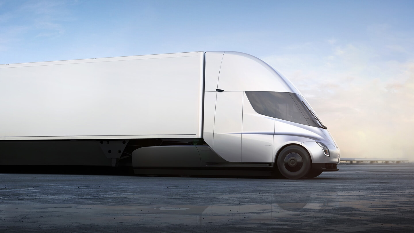
Image source: Tesla

Perfect competition is an abstract idea about how the world would look like when we have unfettered competition. Economists often use perfect competition as a benchmark--a hypothetical state where markets are most effective.

The industry for long-haul trucking illustrates both the advantages of increased competition, but also some of the disadvantages that emerge in practice. Before the 1980's long-haul trucking was heavily regulated by the federal government. A government agency that decided which companies could operate trucks, who could be hired, how much these drivers should get paid and the working conditions for the drivers. Labor unions were strong and being a long-haul trucker was a well-paid job that gave a ticket into the middle class.

The flip side of this was that it was expensive to ship by truck.

But in the 1980's a wave of deregulation happened under the administration of the Republican president Ronald Reagan. The government agency that regulated the trucking industry was abolished and companies were set free in order to compete with each other. A host of new trucking companies were formed, and these companies competed on price, driving down the cost of shipping by truck.

This also meant that the high wages and occupational goods that drivers had enjoyed began to be cut. Not only did wages begin to fall, but hours spent on the open road increased. Many drivers were no longer given the chance to sleep overnight at a motel, but where rather instructed to sleep in their trucks.

Today, long-haul trucking is a job with extremely high churn, that is-a high proportion of workers end up quitting each year. This trend only strengthened after the Covid-19 epidemic has led to a shortage of truckers in many countries. The pressure on drivers can sometimes veer into the dangerous and illegal - companies forcing drivers to drive long periods without adequate rest or sleep.

Being a long-haul driver has become a much tougher job, with lower pay and often difficult working conditions. At the same time, the market for long-haul trucking is experiencing changes.

• Fuel costs make up a large portion of trucking costs, and several new technologies are coming on the market.
• Tesla wants to introduce an electric truck
• Other companies are looking at using hydrogen as a fuel.
• Selv-driving capabilities may also soon be introduced on some trucks.

The effect that these new technologies has on the market for trucking and the drivers is hard to guess at ahead of time, but could be substantial.

In the next several lessons we look at how we can use simple models to analyse how competition affects markets, as well as how "shocks" to those markets can effect both prices and production.

Perfect competition and market supply

Increase market price Reduce market price

Perfect competition and supply

In the figure above we see three panels. The first two represent firms that are producing identical (or very similar) productions-let's say cars.)

I have chosen an industry known to have a lot of competition. While car companies often operate at very large scales and even large companies like the US have only a few car companies, these companies compete globally. VW from Germany, Toyota from Japan and GM from the US all compete in most major economies. New entrants from China are only increasing competition.

While this industry is not what we would call perfect competition, perhaps it is close enough so that a model of perfect competition will give some insights. In particular, we might say that competition leads to market prices that no one producer can deviate much from. If GM and Toyota produce a compact sedan for 25,000 Euro, then VW probably will not be able to see a similar sedan for 35,000 dollars.

With perfect competition we say that firms are price takers. This means that there is a market price that all producers simply have to accept (the horizontal green line in the figure.)

We know in reality that price differences do exist between similar cars. Car companies are experts at differentiating cars to try to appeal to different tastes and types of consumers. By doing this they can try to charge different (higher) prices.

Still, we can simplify and think of this industry as being perfectly competitive. Given a market price, each company decides how much they will produce and sell based on their individual supply curve (which represents the marginal costs of the firm).

If we want to find the market supply curve, we just need to sum up the supply of all the firms. In the figure above, we sum horizontally. The third panel shows the market supply curve.

Press the Increase market price or Reduce market price buttons to see how the market supply changes with different prices.

One thing we notice here is that VW's supply curve is less steep--that means that when the price increases, VW will increase their production by more than Toyota (perhaps because they have more flexible production?). With a higher price, VW will supply a greater share of the market. We say that VW is more price elastic.

Question: What is the marginal cost of all the car companies in equilibrium (where the supply curves meet the price line?

If you analyse the figure a bit you will see that the marginal cost is the same as price in all the figures. Therefor are all the marginal costs for each of the producers also the same! Each company increases competition until their marginal cost is equal to the market price.

Market demand

Increase market price Reduce market price

In this figure we show a representation for market demand.

The first two panels represent demand from individuals or households. Now most people have only one or two cars, so perhaps we can think about this as a group of people in a certain neighborhood.

Earlier in the course we could interpret the individual demand curves as marginal willingness to pay. Basically, we imagined an individual asking whether their utility or enjoyment from buying one more of the good would be more than the purchase price. If yes, then they would buy one more. If not, then I stop buying.

We could apply the same type of thinking to looking at the number of cars sold in a certain neighborhood or town. When there are few cars in a town and no traffic, ample parking, then it is quite attractive to buy a car and the willingness to pay is high. However as more people buy cars, you get more congestion, harder parking and perhaps more taxes and fees to pay as the city government tries restrict car use.

In the figure we again create the market demand curve by summing horizontally across the individual demand curves.

You can press the Increase market price or Reduce market price buttons to see the effect of changes in price on market demand. Again we see that a less steep demand curve will lead to a larger increase in demand when prices fall. Perhaps in the car-crazy US, will a reduction in car prices lead to large increase in demand. While in Japan, with its compact cities and excellent public transportation, the price elasticity of demand will be less.

Market equilibrium

Perhaps you have asked yourself the question: If individual firms can not decide the price in a competitive market, and individual consumers can not decide the price, then who decides the price?

In a command-and-control type economy like the old Soviet Union, or a regulated marked like publicly run health services like that in Great Britain, a government agency decides prices.

But in a competitive market, we have a much more subtle and interesting result. It is the sum of individual demand and firm supply curves that decides what the price is. This is Adam Smith's famous invisible hand theory. That a competitive market, through competition and free flow of information (a customer can always see and compare prices) automatically establishes a market price. Vigiland consumers enforce this market price by quickly snapping up prices that are lower and avoiding producers that try to sell with high prices.

Notice in the figure that where the aggregate supply and demand curves meet, the marginal willingness to pay for all consumers are the same and all the marginal costs of producers are the same. Everyone should be happy with the purchases made. And there are no transactions that were not made that could have made both consumer and producer better off.

Price changes in the market: Covid-19 and the car industry

Something seems a bit strange with the equilibrium we found earlier. In this equilibrium, prices move towards a stable level. But we know that in reality prices move around. How can we explain that?

The answer is that both supply and demand can and will shift.

Let us continue thinking about the market for cars.

When the Covid-19 epidemic happened, there was suddenly little demand for cars. After all, in many places you weren't allowed to go anywhere. Economists would call this a demand shock that shifts the demand curve to the left (negatively).

When society gradually began to open up again, people wanted to get around, yet there were often still restrictions and fears about using public transport and air travel. Demand for cars increased. We would say this was a positive demand shock.

But the epidemic also affected the car companies. When the economy shut down, operating a car factory became harder and more costly. Protection equipment had to be installed, and it was harder to get workers to come to work. This was what we call a supply shock that led to a shift in the supply curve towards the right.

When vaccines became widely available and society opened up again, these companies saw that they were now able to produce cars again with fewer costs. Now we had a positive supply shock. The supply curve shifts to the left.

How did all these changes affect the equilibrium costs?

From a theoretical stand point it can be difficult to say because the equilibrium price is the result of both shifts in demand and supply curves, and when these shifts have opposite effects, then it can be difficult to establish what the total effect is.

Below, we walk through the shifts one by one.

Shift in demand

+ shift in demand - shift in demand

We start with a shift in the demand curve. From the example above, we said that when the Covid-19 hit, we had a negative demand shock for automobiles.

Press the - shift in demand button. The demand curve moves to the left and the equilibrium price is reduced.

Now we can imagine that we are at the point where society is starting to open up again. Press the + shift in demand so that we get a demand curve that now is above the original supply curve. Now we see that equilibrium prices have increased.

Shift in supply

+ shift in supply - shift in supply

Now we see a shift in the supply curve. In the example we told above, we first saw that the companies experienced higher costs when the Covid-19 epidemic egan. This is a negative supply shock. Press the - shift in supply button to see the effect.

The supply curve shifts inward and the equilibrium price rises.

Now we consider the situation where the costs of production are reduced once society open up again. This is a positive supply shock. Press the + shift in supply button and notice that the supply curve shifts out and the equilibrium price is lowered.

Supply- and demand elasticity

Let us say that we are the manager for a grocery store and we want to get a good idea of how demand for different goods changes when the prices change. This will, of course, be important information when deciding if and how much to increase or lower prices.

For example, we could consider bananas and toothpaste. For both of these goods we could analyse our sales data and see how much was sold at different price points. Basically, we could construct a demand curve, and then also estimate the slope of that demand curve - how much will demand change if we change the price slighly.

But when we try to compare these slopes, things get complicated.

We might see that we sell 100 more boxes of toothpase when we lower prices by .10 Euro. And we sell 25 extra kilos of bananas when those prices go down by .10 Euro. But with different units (boxes of toothpaste, kilos of bananas) it is difficult to compare how sensitive each product is to price changes. Plus, we would expect the effect of a change in price to be relative to the total price.

The solution is to use elasticities: We specify both demand and supply elasticity.

Demand elasticity

Demand elasticity can be defined as the percent change in demand when we get a one percent change in price.

Etterspørselselasitet kan vi definere som prosent endring i etterspørsel når vi får en 1 prosent økning i pris.

We can write this as:

$$\frac{\frac{dD}{D}}{\frac{dp}{p}} = \frac{dD}{dp}\frac{p}{D}$$

Where D is demand, dD is change in demand, p is price, and dp is change in price.

Supply elasticity can be written

$$\frac{\frac{dS}{S}}{\frac{dp}{p}} = \frac{dS}{dp}\frac{p}{S}$$

Now if the price of toothpaste is lowered from 2 euro to 1.8 euro and sales increase from 1000 to 1400, then demand elacticity is:

$$\frac{400}{-.2}*\frac{2}{1000} = -4$$

We can interpret this to say that a one percent reduction in price leads to a 4% increase in demand.

If we also see that when the price of apples goes down from 3 euro to 2.7 euro, and sales increase from 200 kilo to 250 kilo, then we can calculate

Hvis vi også ser at når prisen på apples går ned fra 30kr til 27kr per kilo, så øker salget fra 200 kilo til 250 kilo, så kan vi regne

$$\frac{50}{-.3}*\frac{3}{200} = -2.5$$

Which we interpret as a 1% reduction in price leading to a 2.5% increase in sales

And now we can compare the price sensitivity of demand for apples and toothpaste on the same scale.

Quiz

Answer if the following "shocks" lead to a shift in the demand curve or supply curve

Problems

1.) We can write the formulas for global supply and demand for a certain good as:

Supply:

$$x^S = 20 + 0,4*p$$

Demand:

$$x^D = 50 - 0,2*p$$

What are price, p, and quantity, x, in equilibrium?

Show answer

2.) Assume you have demand and supply functions for a good as in problem 1. We then get a positive shift in the demand function. After this shift, when the price is 50 then demand is 60. The slope of the demand function is unchanged. What will the new equilibrium (\(p^*, x^*\)) be?

Show answer

3.) In the short run, demand for electricity is known to be highly inelastic. That is to say that the consumption of electriciity does not tend to change much from day-to-day based on changes in price.

a.) If we draw supply- and demand curves, will the demand curve be steep or flat?

b.) If the market experiences a supply shock - for example that a major power station is shut down for repair, what implication does inelastic demand have for price volatility?

Show answer