Production, Costs, and Supply
"Production Hell": Tesla, growing pains and life at the margin.
When Tesla introudced its Model 3 sedan, it was seen as a make or break production vehicle. It was the first vehicle that Tesla would truly mass manufacture at a scale comparable to the existing mass car manufactureres, and it was planned to have a price point comparable to other sedans: 35,000 dollars.
Electric cars have tended to be more expensive than traditional internal combustion engines because of the cost of the large battery. But on the other hand, they are in terms of the number of parts, simpler and in theory easier to manufacturer.
But the low price Elon Musk had promised for the Model 3 was dependent on quick ramping up of production capacity. Not everything went to play.
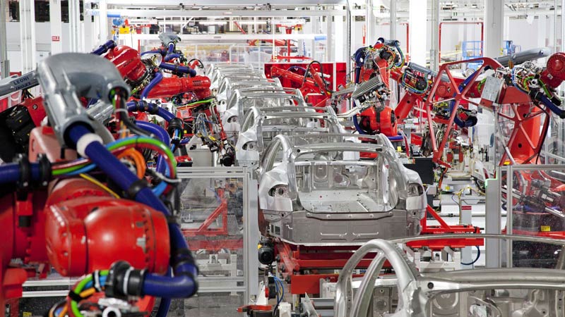
The initial plan was for the factory to be one of the most automated in the world, with much of the assembly job being done by manufacturing robots. But this turned out to be more complicated than expected, and a host of problems emerged because of this overenthusiastic reliance on robots.
Instead Tesla had to pivot to substituting in more manual labor--getting their existing manufacturing employees to work overtime and highering extra personell on short-term contracts. Famously, they even had to setup an extra production line in a tent outside the main factory building.
All of this cost money, and the per-unit cost of the first Model 3s were probably quite high. Tesla likely lost money on each car that was produced in those early days.
But eventually Tesla was able to fix some of the problems in thier production process. They found a better balance between capital (robots) and labor. And most importantly, they were able to learn from their experiences, improve thier production process and bring down unit costs and eventually become profitable.
This part of Tesla's history is about the trade-offs between using labor and capital in production and and how a factory's productivity is related to unit costs. In this lesson we will look more closely at what a microeconomist would have to say about these issues.
The model we will look at is best interpreted as a short-term model where certain factors - like the size or number of factories are fixed. We only consider variable costs in the production process, leaving an analysis of fixed costs for later.
Marginal productivity
The production function, again.
Above, we can again see a production function with diminishing returns to scale. But we will simplify even more than before and consider just one input factor: v, which we will call the resource input. We can think of v as a combined unit of the inputs we need for production. For a car that might be a combination of workers, manufacturing robots, other machines and raw materials. In contrast to our model with labor and capital as inputs, we assume diminishing returns to scale of these resource inputs. We can probably think about this model then as a short-term model where some factors of production are fixed and irrelevant in our model: like the factory building itself for example.
Marginal productivity
An important concept is that marignal productivity. This is the idea of measuring how much extra production you get by adding a little extra resources. In the previous lesson, we considered labor productivity. In this case, marginal productivity was the extra production that came from hiring one more person, or making someone work one hour more.
In this lesson, we will work with a somewhat more abstract concept: How much more production do we get by increasing our resource input by one unit. We could think of it as one worker with tools plus some raw materials. Or even simpler, we could just think of it in monetary terms. One extra euro of inputs will lead to so many more euros of output.
We can perhaps already start to see why this is an important concept. If the resources that go into making one more unit of production cost more than what the product is worth, it probably is not worth making it.
In the figure above, the slope of the green line that goes through the production point represents the marginal productivity.
If you press Increase input we see that the green line represents an approximation to how much we increase production when we increase our input.
Notice as we move up the production curve, the green line becomes flatter: Our marginal production becomes less. Again, this is what we call diminishing returns to scale.
Mathematically, if we write our production as \(y=f(v)\), then we can write marginal production as the derivative of this function with respect to our input, v
$$\frac{dy}{dv} = f'(v) \approx f(v+1)-f(v)$$Average productivity
Average productivity is the idea of taking your total production and dividing by the total amount of inputs used. This will then give an average measure of productivity.
We can write average productivity simply as \(\frac{y}{v}\)
if you press the buttom avg. prod then the read lines show the lengths (v0, y0) that are used to calculate average productivity \(\frac{y0}{v0}\)
The angle of the dotted red line is then our average productivity
By comparing the green and red dotted lines, we can compare average vs. marginal productivity at a certain production point.
The cost function
The cost function
Our cost function is actually just a transformation of our production function.
We begin by flipping our axis so that production (y) is on the horizontal axis and the resource input (v) is on the vertical axis.
We can then give the model the following interpretation? Given a certain production, how much input do we need? If we want to produce 50,000 cars a year, how much inputs do we need?
The only thing we need now is a price on our input
Marginal cost
If you press Increase production Then we can interpret the change in cost (C) as the marginal cost: how much our costs increase if we increase our production by a small amount (for example, 1 unit).
Mathematically, we can write:
$$\frac{dC}{dy} = C'(y) \approx C(y+1)-C(y)$$If you press the button Increase production several times, you can see that marginal costs increase. For each extra unit we produce, the cost of that unit increases somewhat. Does this make sense?
Remember, we are interpreting this model as a short-term model. Given the existing factory, producing more and more units will require our workers to work overtime, running our machines more hours per day, perhaps without sufficient maintenance.
At a longer time scale, we know a producer can reduce their unit costs by increasing scale--investing in newer, larger factories and hiring more workers, but this we will get to later.
Average costs.
Press the Average cost button
We can calculate the average cost (one unit cost) by dividing the total cost by total production..
Mathematically: \(\frac{C(y)}{y}\)
The slope of the red dotted line represents the average cost. By comparing the slope of the green dotted line--the marginal cost--we can see that the marginal cost will always be higher than the average cost in this model. Does this make sense?
The reason is that the marginal cost rises for each extra car that is produced increases. Thus the marginal cost is always above the average cost.
The profit function
Profit and how much to produce
We can use our model and our concept of marginal cost and revenue to decide how much to produce.
First we have to agree on a goal: We want to maximize profit
The figure shows three curves:
- We have our cost curve, which we explained earlier
- Then we have revenues, which is just the price (p) times production.
- So if we produce 50,000 cars which cost 40,000 euro each, then we have a revenue of 2.0 billion euro.
- And then the difference between revenue and costs: profits!
So how much should we produce?
One approach is to try to produce as many cars as possible as long as profits are positive. But then we would end up with close to zero in profits.
Instead press the Increase production button until we are at the top of the profit curve: this is where we maximize profit.
We have also drawn in our marginal cost line: the dotted green line.
At the point of maximum profits, the slope of the dotted green line is the same as the slope of our revenue curve. Is this a coincedence?
NO! The slow of our revenue curve is the marginal revenue, which in this case is just the market price p. Our proft maximizing rule is the following: continue to produce as long as marginal revenue (the revenue of producing one more) is more than the the marginal cost (the cost of producing one more). So a stopping rule is when MR=MC.
Mathematically, letting \(\pi\) represent the profit function, we write:
$$Maks \pi(y) = p*y - C(y)$$ $$\frac{d \pi}{dy} = p - C'(y) = 0$$We maximize profits when: \(p=C'(y)\)
Quiz
Answer True or False about the following statements
Problems
-
Consider the following Cobb-Douglas production function:
$$Y=10*v^{0,5}$$
a.) What is production when v=10 and v=11? What is the difference in production between v=10 and v=11?
b.) What is the marginal productivity when v=10? And when v=20?
c.) What is average productivity when v=10 and when v=20? Is this more or less than marginal productivity?
a.)
When v=10, then production is: \(10*10^{0,5} \approx 31.6\)
When v=11, then production is: \(10*11^{0,5} \approx 33.2\)
The difference in production is: 1.54
Notice that this is our approximate marginal production.
b.)
Now we take the derivative of our production function:
$$f'(v) = 0,5*10*v^{-0,5} = 5*v^{-0,5}$$
We put in 10 and 20 and get:
\(5*10^{-0,5}= 1.58\)
\(5*20^{-0,5}= 1.11\)
This is our exact answer for the marginal production. Notice that the answer for v=10 is quite close to what we found in a.).
Notice also that marginal production goes down when v increases. This is because of diminishing returns to scale in our production function.
c.)
To find the average productivity, we just need to divide our total production with v: \(\frac{f(v)}{v}\). Calculating out:
\(\frac{f(10)}{10}=3.16\)
\(\frac{f(20)}{20}=2.23\)
We notice that average productivity is higher than marginal productivity.
-
a.)Let's say that the price on our resource input is \(q=1\), Write a cost function based on the production function in problem 1.
b.) What is the marginal cost when production is y=25 and y=50?
c.) What is the average cost when y=25 and y=50?
a.) We start with our production function:
$$y=10*v^{1/2}$$We rewrite so that v is on the left side:
$$v^{1/2} = \frac{y}{10}$$ $$v=(\frac{y}{10})^2$$Cost is price times quantity of our input: q*v, so multiplying q by both sides:
$$C = qv = q*(\frac{y}{10})^2 = 1*(\frac{y}{10})^2 = (\frac{y}{10})^2$$b.)
We find marginal cost by taking the derivative of our cost function:
$$C'(y) = 2*\frac{y}{10} = \frac{y}{5}$$
Inserting our values for q and v :
\(\frac{25}{5}=5\)
\(\frac{50}{5}=10\)
Here we see marginal costs rising. It will cost 5 to produce one more when production is at 25, but it will cost 10 to produce one more when production is at 50. This comes from diminishing returns to scale in our production function.
c.)
To find average cost we divide total cost by total production.
\(\frac{C(y)}{y}=\frac{(\frac{y}{10})^2}{y}=\frac{y}{100}\)
\(\frac{25}{100} = 0,25\)
\(\frac{50}{100} = 0,50\)
We notice that average cost is less than marginal cost.
-
Assume we have a cost function as in Problem 2.
a.)Assume the market price for our good is 2, how much should we produce?
b.)The market price rises to 3, how much should we produce now?
a.) If we want to maximize profit, then we should start with our profit function:
$$\pi(y) = p*y-C(y)$$We put in our cost function C(y)
$$\pi(y) = p*y-(\frac{y}{10})^2$$The maximum is where the marginal profit is 0 (producing one more will give 0 in profit)
$$\pi'(y) = p-\frac{y}{5}=0$$Our condition for maximum profit is:
$$p=\frac{y}{5}$$(MC=p)
When p=2:
\(2=\frac{y}{5}\)
y=10
b.)When p=3:
\(3=\frac{y}{5}\)
y=15, we increase production when the price rises.)